Solving a facility location problem in near-linear time

0. Problem Description

Given a list of household locations $0 \le A[1] \le \cdots \le A[n]$ and candidate facility locations $0 \le B[1] \le \cdots \le B[m]$. Your task is to place $k$ hospitals, i.e. choose a subset $S \subseteq \{1, 2, \dots, m\}$, such that $\sum_{1 \le i \le n} \min_{j \in S} |A[i] - B[j]|$ is minimized. In other words, if we add up the minimum distance to a household to any of the chosen hospitals, the sum should be the minimum possible.

I. Basic solution

One key observation is that people going to the same hospital must live in neighbouring locations. The proof is as follows:

If someone on your left and someone on your right are both choosing the same hospital $x$, you should go to the same one as well. If you go to any hospital $y$ that is left of $x$, it would be better for that person on your left to go to hospital $y$ as well. Similarly for going to a hospital that is right of $x$.

Therefore, we can formulate this problem as partitioning the people into (at most) $k$ contiguous sections, then assigning a hospital to each section, so that the total distance is minimized.

With this in mind, we define the dp states as follows:

Definition 1 (DP states):
Let $cost(l, r)$ be the minimum total distance for people $l$ to $r$, if we assign them to the same section (same hospital).
Let $dp[i][j]$ be the minimum total distance for people $1$ to $j$, if we assign them to $i$ sections.

The decision for $dp[i][j]$ would be where to start the $i$-th section (we know that it ends at $j$). Thus we arrive at the recurrence

If we implement this recurrence straightforwardly, the runtime would depend on the time needed to compute $cost(\cdot, \cdot)$ function. The baseline is $O(nm)$ per query: try all $m$ hospital locations and compute total cost in $O(n)$ time. This leads to a solution with overall runtime $O(kn^3m)$.

Below we describe a few optimizations:

• Precomputation: We can precompute $cost(l, r)$ for all $l$ and $r$, to avoid repeated computations in the dp recurrence.
• Prefix sum/partial sum: We can compute the total distance to a specific hospital (say at $x$) for people $l$ to $r$ in $O(1)$ time, using prefix sum. The idea is that there is a break-off point $p^* \in [l-1, r]$ so that people $l$ to $p^\*$ are to the left of $x$ and people $p^* + 1$ to $r$ are to the right of $x$. Then, the sum becomes $\sum_{i=l}^{p^*} (x - a[i]) + \sum_{i=p^*+1}^r (a[i] - x)$, which can be computed in $O(1)$ with a prefix sum on the $a[i]$ array and if $p^*$ can be found in $O(1)$ (how?).
• Median: for a contiguous section of people $l\dots r$, if we can build a hospital freely, then choosing a median of the locations $a[l], \dots, a[r]$ would be optimal (proof left as exercise). By extension, we should choose either the location that is immediately to the left of the median, or immediately to the right of the median. We don’t need to consider all $m$ candidate locations.

Using either of the observations, the overall runtime can be reduced to quartic, e.g. $O(kn^2m)$ using (1). By combining at least two of the three observations, you can get the overall runtime down to cubic or nearly cubic, e.g. $O(kn^2 + n^2 m)$ by combining (1) and (2).

II. Divide and conquer…?

It turns out that using an advanced optimization technique, called the “Divide and Conquer optimization” in the competitive programming community, we can obtain a solution with runtime $O(kn \log n + n(n+m))$, i.e. nearly quadratic!

First, precompute $cost(l, r)$ for all $l, r$ in $O(n(n+m))$ time. This can be done by combining all the three optimizations.

Now, on to the DP part. We will fill the DP table row by row. The goal is to compute $dp[i][0..n]$ given $dp[i-1][0..n]$ in $O(n \log n)$ time. Since we need to do this $k$ times, the overall runtime (taking into account the precomputation) will be $O(kn \log n + n(n+m))$.

The idea here is to use an additional solution structure: monotonicity of the optimal subproblem. Let me first present formally:

Proposition 2 (monotonicity of optimal subproblem)
Let $opt[i][j]$ be the smallest index $l$, such that $dp[i-1][l] + cost(l+1, j)$ is minimized. Then, $opt[i][1] \le opt[i][2] \le \cdots \le opt[i][n]$.

In other words, if it is optimal to group people $l...j$ in an $i$-group arrangement, and if it is optimal to group people $l'...j+1$ in an $i$-group arrangement, then $l \le l'$. The key element of the proof is that the cost function satisfies the quadrangle inequality: for $a \le b \le c \le d$, $cost[b][c] + cost[a][d] \ge cost[b][d] + cost[a][c]$. The proof is not very easy. If you want to check your proof or know how it’s done, please reach out to me.

With this, we can prove the monotonicity of optimal subproblem. Suppose on the contrary that $opt[i][j] > opt[i][j+1]$ for some $j$. By definition of $opt$ we have:

1. $dp[i-1][opt[i][j]] + cost[opt[i][j]+1][j]$ $< dp[i-1][opt[i][j+1]] + cost[opt[i][j+1]+1][j]$

2. $dp[i-1][opt[i][j+1]] + cost[opt[i][j+1]+1][j+1]$ $\le dp[i-1][opt[i][j]] + cost[opt[i][j]+1][j+1]$

Adding up the two, and cancelling common terms on both sides of the inequality, we get $cost[opt[i][j]+1][j] + cost[opt[i][j+1]+1][j+1]$ $< cost[opt[i][j+1]+1][j] + cost[opt[i][j]+1][j+1]$. Taking $a=opt[i][j+1]+1, b=opt[i][j]+1, c=j, d=j+1$, this becomes $cost[b][c]+cost[a][d] < cost[b][d] + cost[a][c]$, which is a violation of the quadrangle inequality.

Let me give you an idea of why this property would help. Short answer: to reduce search space.

Without this monotonicity property, one would need to go through subproblems $dp[i-1][0..j]$ to calculate $dp[i][j+1]$. But suppose you know that $opt[i][j]=t$. Then we only need to go through $dp[i-1][t..j]$ to calculate $dp[i][j+1]$.

There is one small issue: if $t$ turns out to be really small, then it appears to be ineffective in narrowing the search range. However, notice that we can use it to narrow the search range for $dp[i][j-1]$: we only need to go through $dp[i-1][0..t]$ to calculate $dp[i][j-1]$!

To calculate $dp[i][l..r]$, let $mid := (l+r)/2$, and let $t := opt[i][mid]$. Then, to calculate $dp[i][l..(mid-1)]$ we only need to look at subproblems $dp[i-1][0..t]$, and to calculate $dp[i][(mid+1)..r]$ we only need to look at subproblems $dp[i-1][t..r]$. We do this recursively to further narrow the search range — divide and conquer :)

For the implementation, you can refer to Slides 67-72 of this presentation (external link) which I made a few years back. The slides use $C[i][j]$ instead of $opt[i][j]$.

III. Faster than quadratic

This is not the end of the story. In fact we can solve the problem in time $O(n \log n \log RANGE)$!! If you turn a blind eye to those logs, there is only one lonely $n$ term left… (Why is this surprising? Well, even the number of states of the DP is quadratic, so how can the runtime be less than that?)

This magic trick is called the “Aliens trick” in competitive programming community. It is useful for eliminating one of your DP state dimensions. In the context of this problem, the idea is as follows:

• Instead of keeping track of number of sections (= number of hospitals) so far, assign a penalty $\lambda$ to each section (i.e. it costs $\lambda$ to build a hospital), and hope that in the end the number of sections will be equal to $k$.

So, let $dp_{\lambda}[i]$ be the minimum total cost for people $1$ to $i$, if we assign them into any number of sections, but each section increases the cost by $\lambda$. Then,

Claim 1: We can compute $dp_{\lambda}$ in $O(n \log n \log m)$ time

Claim 2: We can find a suitable $\lambda$, by computing $dp_{\lambda}$ for $O(\log RANGE)$ different values of $\lambda$. $RANGE$ is the range of the input numbers

For claim 1, let me refer you to this tutorial (external link). Again, the algorithm works because the cost function satisfies the quadrangle inequality. The quadrangle inequality means that, once subproblem $l$ is dominated by some later subproblem (i.e. $opt[i][j] > l$ for some $j$), it will not be optimal anymore (i.e. $opt[i][j'] > l$ for all $j' \ge j$). The method in the tutorial essentially looks to maintain the set of “active” subproblems.

We need to compute the cost function $O(n \log n)$ times, each computation taking $O(1)$ time (combining optimizations 2 and 3; note that it is too slow to precompute the cost functions!). The runtime is therefore $O(n \log n)$.

For claim 2, refer to this diagram below:

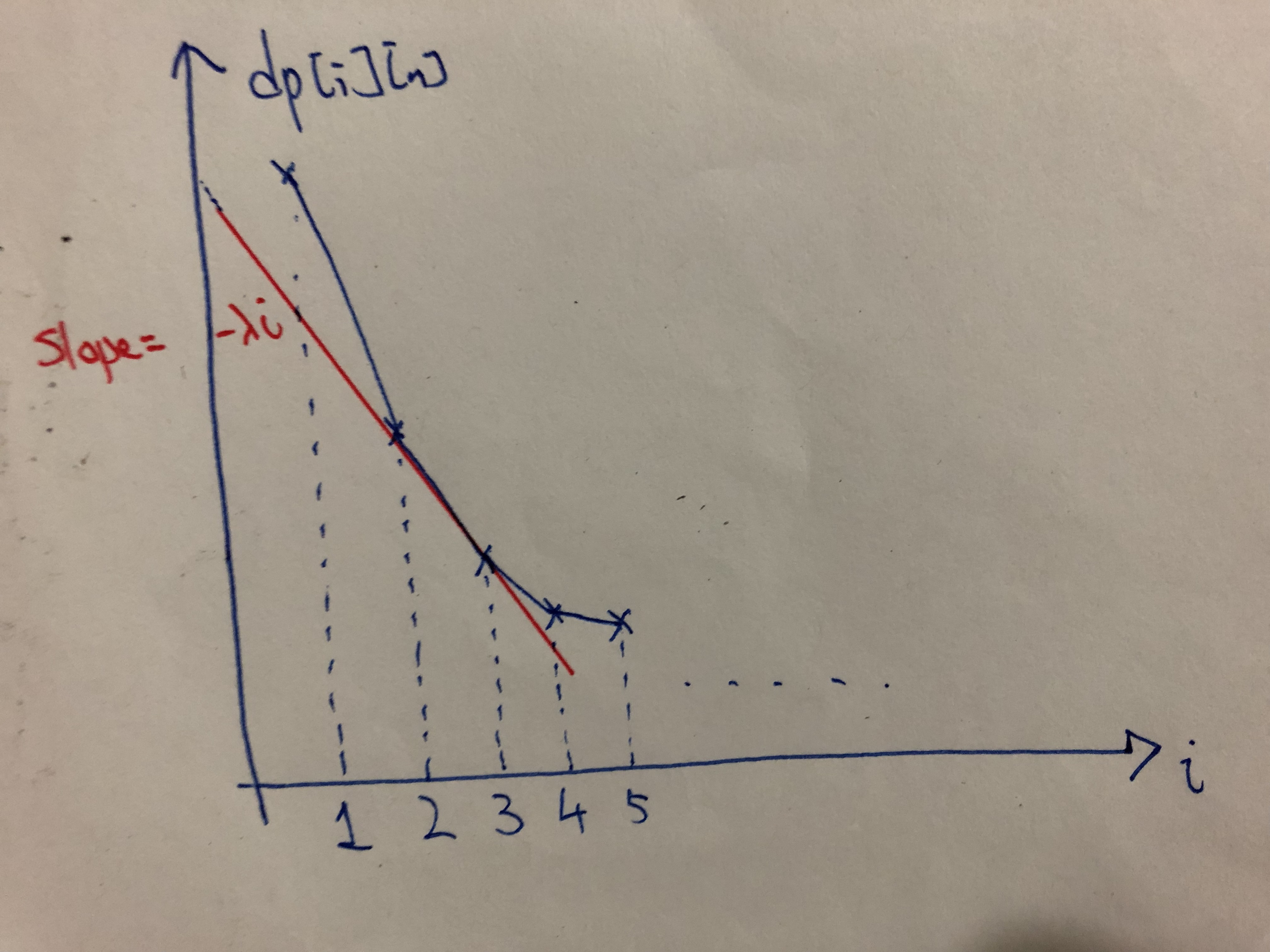
Varying $\lambda$ is akin to varying the slope of the red line, and the point that is “closest” to the line corresponds to the optimal number of hospitals $i$. Let’s consider extremal examples: when $\lambda$ is very big, the cost of building a hospital is high, so it should be optimal to have $i=1$. When $\lambda$ is zero, there is no cost to build a hospital, so it should be optimal to have $i=m$ (build hospitals at all candidate locations).

If the function $i \mapsto dp[i][n]$ is convex (i.e. the graph above is convex), then by varying $\lambda$ we can make all different values of $i$ optimal (or one of the optimal), and we can binary search on $\lambda$ to find the $\lambda$ so that building $i=k$ hospitals is optimal. Binary search would take $O(\log RANGE)$ iterations (note that we only need to check integer values of $\lambda$), and in each iteration we would compute $dp_\lambda$ for some $\lambda$.

To check convexity of $i \mapsto dp[i][n]$, check that $dp[i-1][n] + dp[i+1][n] \ge 2 dp[i][n]$. The idea is that, given an optimal partition $C_{i-1}$ into $i-1$ groups and an optimal partition $C_{i+1}$ into $i+1$ groups, we can construct two partitions $C_i$ and $C_i'$, both into $i$ groups, so that their sum of costs is at most the sum of costs of $C_{i-1}$ and $C_{i+1}$ (this step uses the quadrangle inequality).

Therefore, we have an $O(n \log n \log RANGE)$ solution to the facility location problem.

IV. Afterword

Dynamic programming is a powerful algorithm paradigm. This course has shown you the basic examples and ideas that help demystify DP and turn it from magic to craft, something that you can reliably use to tackle problems. Hopefully, this writeup has given you a glimpse of the beautiful ideas and techniques that DP incorporate, to show that DP is not just a craft, but also an art.